Weather Station
- Introduction
- Background
- Hardware Setup
- Code Layout
- Configuration
- Firmware Implementation
- Classification
- Showcase
- Developer Notes
Introduction
Weather Station is a project intended to demonstrate the usage of barometric air pressure DPS368 and humidity SHT40-AD1F sensors on the SensEdu shield.
This turns the board into a small environmental measurement station that reports temperature, humidity, dew point, and sea-level pressure every few seconds, along with classifications of each quantity. The station also tracks how the sea-level pressure changes over time and reports a simple forecast of the improving or worsening of the conditions.
Background
This section presents what some of the measured quantities mean and why they are useful for determining the environmental conditions.
Humidity
Humidity is the amount of water vapor in the air. It could be represented in three different ways.
Absolute Humidity (AH)
The mass of water vapor per volume of air.
Specific Humidity (SH)
Intuitively, AH feels like the right metric to describe the absolute water vapor in the air, but it is actually true only if the volume is constant as well (imagine sealed rigid container).
But in the case of open air which is more typical for meteorological measurements, volume is not constant. For example, heating up the air at typical atmospheric pressure makes it expand, which leads to the same mass of vapor spreading through a larger air volume, so absolute humidity actually decreases.
Therefore, there exists another vapor metric which is independent of volume changes called specific humidity (SH), defined as the mass of water vapor per unit mass of moist air.
Relative Humidity (RH)
Defined as the ratio of the current water-vapor content to the maximum the air could hold at the same temperature, expressed as a percentage.
RH depends on both water vapor content and temperature: warmer air can hold more water, meaning heating the air with certain specific humidity will actually lower its RH even though no water has been removed. Conversely, cooling the air will raise its RH.
This brings us to the main caveat of RH — it is not a great way to determine how the humidity feels to a person. Much of our perception of humidity comes from how easily sweat can evaporate from the skin. For this reason, the dew point is a more intuitive measure of perceived humidity than RH.
Dew Point
Dew point is the temperature to which the air would have to be cooled (at constant specific humidity) for it to start condensing into dew or fog. Unlike RH, the dew point is an absolute property of the air’s water content, expressed in °C. Two different air samples with the same dew point hold the same amount of water vapor regardless of their current temperatures or RH. It helps avoid misleading humidity decisions just based on the RH, which can change with temperature even if the specific humidity is constant.
This metric makes for a useful comfort indicator, tracking the actual moisture content of the air, which is what makes it feel sticky or dry. You can read more about the relation to human comfort here.
To calculate the dew point from the sensor readings, the Magnus formula is usually used, expressed as:
\[\gamma(T, RH) = \ln\!\left(\frac{RH}{100}\right) + \frac{aT}{b + T}\] \[T_d = \frac{b \cdot \gamma(T, RH)}{a - \gamma(T, RH)}\]- \(T_d\) – dew point (°C)
- \(T\) – temperature (°C)
- \(RH\) – relative humidity (%)
- \(a = 17.625\), \(b = 243.04\) °C – empirical fitting constants, optimized for the range −40 °C to +50 °C
Dew Point Depression
Dew point depression \((T − T_d)\) is the difference between the temperature and dew point temperature. A small dew point depression indicates that the air is close to saturation, which can lead to the formation of fog or mist. Respectively, a large dew point depression indicates that the air is relatively dry and less likely to produce condensation.
Atmospheric Pressure
Atmospheric pressure is the force per unit area that the atmosphere exerts on the Earth’s surface, caused by the weight of the air above. You can find a more detailed explanation here. The important thing is that pressure gradients are a main driver of weather patterns. Air drifts across regions, and changes in pressure are directly associated with different weather conditions.
As a rule of thumb, high pressure is associated with clear skies and calm conditions, while low pressure is associated with clouds and precipitation. Since high and low pressure are relative concepts, a reference value was defined, called the standard sea-level pressure of 1013.25 hPa measured at 0 altitude.
Since the pressure decreases with altitude, a raw reading from a station at, say, 500 m above sea level cannot be compared directly against the sea-level reference. For that reason, the standard way is to recalculate the pressure to its sea-level equivalent using the location altitude and the current temperature. This way, the reading can be compared against the reference and classified properly.
Calculation is done using the barometric formula:
\[P_0 = P \cdot \left[\frac{T}{T_0}\right]^{\dfrac{g'_0 M_0}{R^* L}}\]- \(P_0\) – sea-level equivalent pressure (Pa)
- \(P\) – pressure at weather station (Pa)
- \(T\) – temperature at station (K)
- \(T_0\) – temperature at sea level (K)
- \(L\) – temperature lapse rate (K/m); \(-6.5\) K/km at sea level
- \(h\) – station altitude (m)
Temperature at sea level (\(T_0\)) can be calculated by extrapolating from the station temperature (\(T\)) using the lapse rate:
\[T_0 = T - L \cdot h = T + 0.0065 \cdot h\]The exponent is a constant:
\[\dfrac{g'_0 M_0}{R^* L} = \dfrac{9.8\,\text{m/s}^2 \cdot 0.03\,\text{kg/mol}}{8.31\,\text{J/(mol·K)} \cdot (-6.5\,\text{K/km})} \approx -5.257\]- \(g'_0\) – standard gravity (9.80665 m/s²)
- \(M_0\) – mean molar mass of air at sea level (28.9644 kg/kmol)
- \(R^*\) – universal gas constant (8.31432 J/(mol·K))
Thus, the formula simplifies to:
\[P_0 = P \cdot \left[\frac{T}{T + 0.0065 \cdot h}\right]^{-5.257} = P \cdot \left[1 + \frac{0.0065 \cdot h}{T}\right]^{5.257}\]Do not forget to convert degrees Celsius to Kelvin by adding \(273.15\) to the station reading.
After proper conversion the pressure can be classified as high or low. But rather than flat labels, the much more useful information is the pressure trend over the last few hours. This is what actually predicts in which direction the weather is developing. A rising trend is associated with improving conditions, while a falling trend is associated with worsening conditions and higher chances of precipitation.
There is a classic forecasting nomogram called Zambretti Forecaster which predicts weather based on current pressure and the pressure trend. It claims to be 94% accurate when calibrated in its home UK climate.
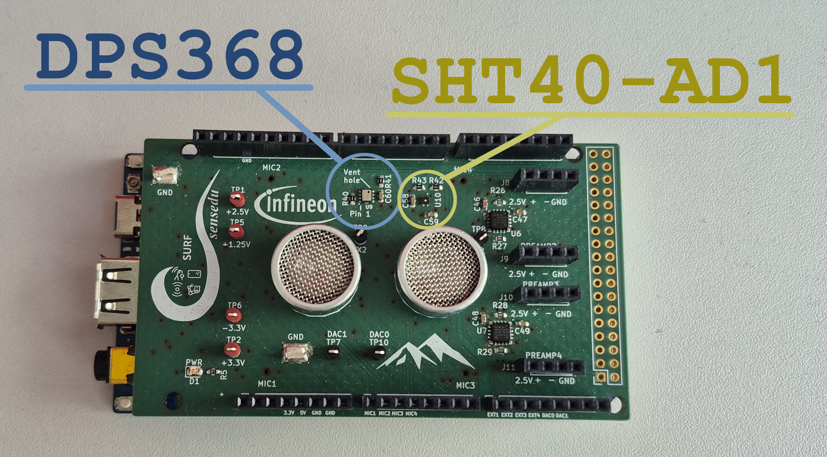
Hardware Setup
Connect the shield to Arduino GIGA R1 as usual, and access both DPS368 and SHT40-AD1F sensors via the primary I2C bus at pins 20 (SDA) and 21 (SCL).
To use the primary I2C bus you need to include the Wire library in Arduino sketch and call the Wire.begin() in the setup function.
Ensure to use Wire specifically, not the Wire1 or Wire2. They refer to different I2C buses. Refer to Arduino GIGA R1 I2C section in the documentation for more details.
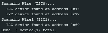
For I2C communication each sensor has assigned address. The DPS368 uses 0x77 and the SHT40-AD1 0x44. You can verify it and the basic communication in general via an I2C scanner sketch (see Developer Notes), which is provided in the projects/Weather_Station/scanner/ directory. The expected output should show both addresses as active on Wire bus.
Communication is actually established by the third-party sensor libraries, which are included as dependencies in the sketch. The libraries handle all low-level I2C transactions, so the weather station just calls their high-level APIs to get the measurements.
- Infineon DPS368:
arduino-xensiv-dps3xx. - Sensirion SHT40-AD1:
arduino-i2c-sht4x
SHT40-AD1 library example has a problem with its compilation on Arduino GIGA R1. The patched one is available in the projects/Weather_Station/sht4x_example/ directory, and the issue is described in more detail in the Developer Notes section below.
Code Layout
The sketch is split into multiple .ino files. Arduino concatenates them all together at compile time, so they share global state without explicit #includes between them. The shared types live in a real .h header for proper include order.
| File | Purpose |
|---|---|
Weather_Station.ino
| Entry point. Holds all user-tunable #define macros, the global sensor objects, setup(), and loop(). The loop performs one read + compute + display cycle.
|
sensors.ino
| Three measure_*() wrappers that call the libraries and return false on error. Pure I/O.
|
metrics.ino
| All math (sea-level pressure, dew point) and all printing (each report_*() formats one row of the serial dashboard, with a classify_*() helper for the readable status label).
|
pressure_trend.ino
| Implements pressure trend. A circular buffer captures one sea-level pressure sample every PRESSURE_PERIOD_MIN minutes; try_get_pressure_trend() runs a least-squares regression over the recent window.
|
pressure_types.h
| The two structs (PressureSample, PressureTrendStatus) shared between the trend sketch and the report printer.
|
Configuration
All knobs live as #define macros at the top of Weather_Station.ino:
| Macro | Default | Meaning |
|---|---|---|
DEBUG_WAIT_FOR_SERIAL
| 0 | Set to 1 to make setup() block until a serial monitor connects. Useful when debugging setup().
|
ALTITUDE_M
| 501.0 | Station altitude above mean sea level, in meters. |
DISPLAY_PERIOD_SEC
| 5 | Seconds between display refreshes. Sensor reads happen at this same rate. |
PRESSURE_PERIOD_MIN
| 30 | Minutes between captures into the pressure-trend buffer. The trend window length is PRESSURE_PERIOD_MIN * PRESSURE_TREND_SAMPLES.
|
PRESSURE_HISTORY_SIZE
| 48 | Total slots in the circular history buffer (24h with the defaults). |
PRESSURE_TREND_SAMPLES
| 6 | Number of recent samples the regression uses. Together with PRESSURE_PERIOD_MIN defines the trend window (3h with the defaults).
|
SHT_AS_TEMP_SOURCE
| 1 | Which sensor’s temperature reading is used as “ambient” for display. Dew point itself always uses the SHT (see Developer Notes). |
DPS_OVERSAMPLING_RATE
| 5 | DPS368 oversampling exponent (0–7). The sensor takes \(2^N\) internal samples per result; more accurate but slower. |
DPS_TEMP_OFFSET
| −3.0 °C | Empirical offset subtracted from the DPS temperature to compensate for self-heating on this PCB. |
SHT_TEMP_OFFSET
| −2.5 °C | Same, for the SHT4x. |
Ideally, the offsets should be determined experimentally with a known-good reference thermometer in the same environment as the station.
Firmware Implementation
This section will describe the general idea behind the firmware implementation. Refer to the full source code under /projects/Weather_Station/ for the complete picture.
Sensor Initialization
There is one global object for each sensor. The setup() function then calls their begin() methods directly as described in examples by the respective libraries.
#include <Dps3xx.h>
#include <SensirionI2cSht4x.h>

SensirionI2cSht4x sht_sensor;
Dps3xx dps_sensor = Dps3xx();

void setup() {
    Wire.begin();
    Serial.begin(9600);
    dps_sensor.begin(Wire);
    sht_sensor.begin(Wire, SHT40_I2C_ADDR_44);
    sht_sensor.softReset();
    delay(10);
}
Measurements
The measure_*() functions in sensors.ino are simple wrappers around the library calls that return false on any error, so the main loop can decide how to handle it. Example for DPS368 temperature measurement:
bool measure_dps_temp(float* temp) {
    int16_t err = dps_sensor.measureTempOnce(*temp, DPS_OVERSAMPLING_RATE);
    if (err != 0) {
        Serial.print("Failed DPS Measurement. DPS lib error code: ");
        Serial.println(err);
        return false;
    }
    return true;
}
Main Loop
- Raw data acquisition from both sensors: No offsets are applied yet. If any sensor errors out, the cycle is aborted.
- Dew point calculation: Magnus formula applied to the raw SHT temperature/humidity pair. The SHT is always used here, since the dew point requires T and RH from the same physical state of the air — using a matched pair from the same sensor improves accuracy (see Developer Notes).
- Ambient temperature: The empirical offset configured by the user is applied to get a corrected ambient temperature, rather than taking the temperature exactly at the sensor point on the PCB.
- Ambient relative humidity: Recomputed from the corrected ambient temperature and the (already-locked-in) dew point, using the Magnus formula in reverse (see Developer Notes). This is the RH a person standing next to the device would experience, not the RH at the sensor surface.
- Dew point depression: The dew point is subtracted from the ambient temperature.
- Sea-pressure conversion: Recomputation of the pressure reading to equivalent sea-level pressure using the ambient temperature and specified altitude.
- Fill the pressure trend buffer: At configured intervals the sea-level pressure is saved into the circular buffer.
- Pressure trend calculation: If enough samples have been collected, the trend is computed via least-squares regression.
- Print the dashboard: All values are displayed in three columns: metric label, value, and classifier tag.
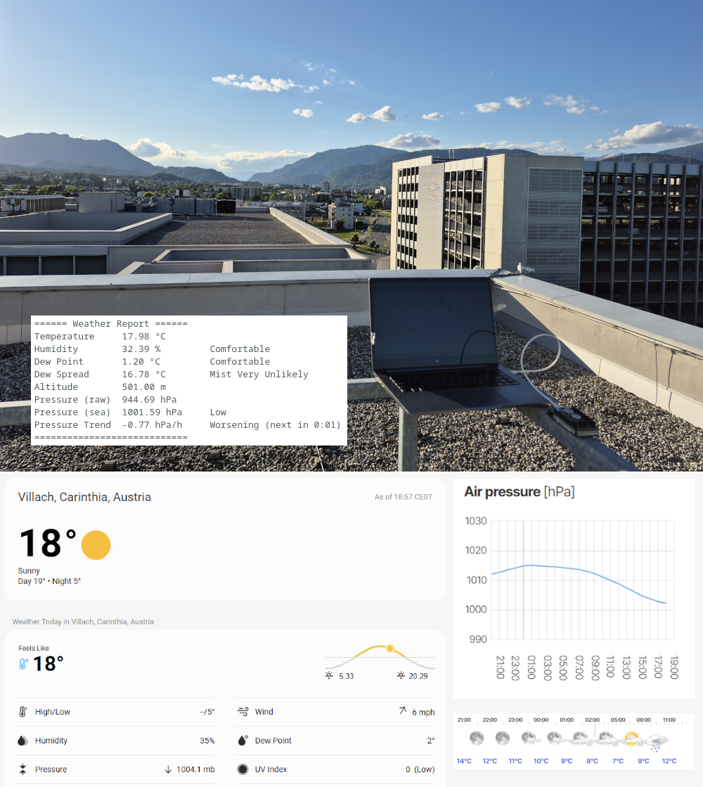
The full output of one cycle looks like this:
====== Weather Report ======
Temperature     22.43 °C
Humidity        48.54 %         Comfortable
Dew Point       11.05 °C        Comfortable
Dew Depression  11.38 °C        Fog Unlikely
Altitude        501.00 m
Pressure (raw)  954.32 hPa
Pressure (sea)  1015.78 hPa     Normal
Pressure Trend  -0.42 hPa/h     Worsening (next in 0:14)
============================
Classification
Each measured quantity is mapped to a short human-readable label by a small classify_* helper in metrics.ino. I attempted to find the standard for each of the metrics and assign them accordingly.
Relative Humidity
As discussed above, labeling RH is not straightforward — it is heavily affected by temperature, so the same value can feel very different on a cold morning versus a hot afternoon. It is most meaningful indoors, where room temperature stays relatively stable. For that reason, formal guidance only defines the comfortable range; the surrounding bands are informal extensions.
The “Comfortable” band is taken from the US EPA indoor air quality guidance, which recommends keeping indoor RH below 60%, ideally between 30% and 50%.
| Relative Humidity (%) | Project Label |
|---|---|
| < 30 | Dry |
| 30–60 | Comfortable |
| 60–75 | Humid |
| 75–90 | Very Humid |
| ≥ 90 | Saturated |
Dew Point
Dew point maps fairly directly onto perceived comfort — better than relative humidity, since it’s an absolute measure of moisture in the air.
The structural source is the Australian Bureau of Meteorology. It offers a six-band scale calibrated for Brisbane’s humid subtropical climate. BOM’s thresholds somewhat line up well with what the Deutscher Wetterdienst describes for Central Europe. Specifically, a “Schwülegrenze” (sultriness threshold) is defined around 16–17 °C, and ≥ 20 °C is said to be “ziemlich unangenehm” (quite unpleasant).
Two adjustments have been made — dew points above ~22 °C are essentially never seen in Central Europe, so BOM’s upper “Oppressive” band is pulled down. At the same time, the lower bands are relabelled upward. What BOM calls “dry” is normal in Central Europe’s drier baseline climate, so the project treats lower range as “comfortable.”
| Dew Point (°C) | Project Label | BOM (Brisbane) |
|---|---|---|
| < 5 | Dry | Very dry |
| 5–15 | Comfortable | Dry (BOM: 5-10); Comfortable (BOM: 10-15) |
| 15–20 | Muggy | Starting to feel muggy (BOM: 15–20) |
| 20–22 | Oppressive | Muggy and quite uncomfortable (BOM: 20–24) |
| > 22 | Miserable | Oppressive (BOM: > 24) |
Climate acclimatisation matters. People adapted to more humid climates tolerate higher dew points; Central Europeans are accustomed to a drier baseline than Australians and may find discomfort sets in earlier than the BOM scale suggests.
Dew-point Depression
Dew-point depression (also called spread) can be used to estimate the likelihood of fog formation. The smaller the spread, the closer the air is to saturation and the higher the chances of condensation occurring. The 2.5 °C threshold is given by the NWS fog guide.
| Spread (°C) | Label |
|---|---|
| < 2.5 | Fog Likely |
| ≥ 2.5 | Fog Unlikely |
Sea-level Pressure
The standard sea-level pressure of 1013.25 hPa is defined by the International Standard Atmosphere. The “Normal” band contains the reference value. For the surrounding bands I used 10 hPa steps based on my measurements and comparison with weather at my location and also partially derived from labels used in Zambretti Forecaster.
| Pressure (hPa) | Label |
|---|---|
| ≥ 1030 | Very High |
| 1020–1030 | High |
| 1010–1020 | Normal |
| 1000–1010 | Low |
| 990–1000 | Very Low |
| 980–990 | Extremely Low |
| < 980 | Storm |
Pressure Trend
Pressure tendency is a key predictor of weather changes. A rising pressure usually indicates improving weather, while a falling pressure suggests worsening conditions and higher chances of precipitation. The named categories come from the UK Met Office shipping forecast terminology, as documented by All At Sea, which gives fixed three-hourly amounts for four of the six categories:
- slowly (0.1–1.5 mb)
- rising/falling (1.6–3.5 mb)
- quickly (3.6–6.0 mb)
- very rapidly (> 6.0 mb)
This project measures pressure changes in hPa/h, so the above amounts are divided by 3 to get the per-hour equivalents. A “Steady” band is added around zero to avoid over-sensitivity to small fluctuations. “Improving” and “Worsening” span the normal rising/falling range; “Clearing” and “Storm Incoming” cover both the quickly and very rapidly changing conditions, in the rising and falling directions respectively.
| Trend (hPa/h) | Label |
|---|---|
| > +1.2 | Clearing |
| +0.5 … +1.2 | Improving |
| −0.5 … +0.5 | Steady |
| −1.2 … −0.5 | Worsening |
| < −1.2 | Storm Incoming |
Showcase
Do not measure under direct sunlight or near a heat source, as it will bias the temperature readings and thus all the derived metrics. The station is designed to be used in the shade or indoors.
If you find your readings being off from official weather reports, sometimes it can be expected in your specific measuring conditions. For example, the temperatures are generally higher close to the buildings. Most comparable conditions are usually in open air, e.g. on the roof or open field.
The station was tested at Villach, Austria (501m) at 19:00 CEST on 13.05.2026, during a clear sky day with a light breeze and coming heavy rain later.
Developer Notes
SHT4x Example Compilation Error
The example arduino-i2c-sht4x/examples/exampleUsage/exampleUsage.ino shipped with the Sensirion SHT4x library does not compile out of the box on the Arduino GIGA R1.
The compiler says:
error: 'int16_t error' redeclared as different kind of symbol
 static int16_t error;
                ^~~~~
note: previous declaration 'void error(const char*, ...)'
 MBED_NORETURN void error(const char *format, ...) MBED_PRINTF(1, 2);
                    ^~~~~
The problem is that the example declares a file-scope variable named error which already exists in Mbed Arduino Core at mbed_error.h. Both symbols live in the global namespace, so the compiler refuses to compile the sketch. The example is fixed in the patched copy under projects/Weather_Station/sht4x_example/ by renaming SHT error variable to sht_error.
Relevant Pull Request.
I2C Scanner
The typical Arduino I2C scanner found online cannot detect the SHT4x on Arduino GIGA. The classic pattern relies on a zero-byte write to probe each address, which works for most sensors including DPS368, but SHT4x is a command-driven sensor that will not ACK unless a valid command byte is received. The reliable workaround is to send a 1-byte write of a dummy value and accept as “device present” both I2C_OK (device ACKed everything) and I2C_ERR_DATA_NACK (address ACKed but data byte NACKed).
A scanner that uses this probe and walks both Wire and Wire1 is provided under projects/Weather_Station/scanner/.
Dew Point Calculation
Two subtle pitfalls when computing dew point from sensor data:
Do not apply the empirical temperature offset before calling the Magnus formula.
The DPS_TEMP_OFFSET / SHT_TEMP_OFFSET constants in Weather_Station.ino exist to compensate for sensor self-heating. When a sensor self-heats, its temperature reading rises and its humidity reading falls as well. The two shift together so that the dew point derived from the pair remains correct.
The (T, RH) pair is self-consistent and feeds Magnus a physically valid state. If you apply the offset before dew point computation, you lower the temperature while leaving the humidity unchanged, breaking that pairing and biasing the computed dew point a few degrees too low.
Always use the SHT temperature, not the DPS temperature.
The Magnus formula assumes T and RH describe the same physical state of the air. The SHT4x measures both quantities from the same silicon die at the same instant — a guaranteed-consistent pair. Mixing the DPS368’s temperature reading with the SHT4x’s humidity reading combines two sensors with different self-heating profiles, mounted on different parts of the PCB, sampled at slightly different times.
The SHT_AS_TEMP_SOURCE macro in Weather_Station.ino controls only which sensor provides the displayed ambient temperature (and feeds the sea-level pressure conversion).
Ambient RH
Ambient temperature is acquired by subtracting the empirical offset from the raw sensor reading. Relative humidity cannot be corrected the same way — it depends on temperature, so simply subtracting an offset from the raw RH value would give a wrong result. The correct approach is:
- Read raw SHT temperature and humidity
- Compute dew point from the raw
(T, RH)pair. This locks in the air’s specific humidity. - Apply the temperature offset to obtain the corrected ambient temperature.
- Recompute relative humidity from the corrected temperature and the dew point (invert the Magnus formula). This gives the RH the air actually has at the ambient temperature, not the RH the hot sensor surface saw.
The main principle behind is that dew point is a property of the air’s specific humidity. It does not depend on the sensor’s temperature, the displayed temperature, or any offset. Once it has been derived from a self-consistent raw measurement, it becomes the anchor for everything moisture-related.